Drawing subgroups of the modular group

Previously we learned how to count the finite index subgroups of the modular group . The worst thing about that post was that it didn’t include any pictures of these subgroups. Today we’ll fix that.

The pictures in this post can be interpreted in at least two ways. On the one hand, they are graphs of groups in the sense of Bass-Serre theory, and on the other hand, they are also dessin d’enfants (for the rest of this post abbreviated to “dessins”) in the sense of Grothendieck. But you don’t need to know that to draw and appreciate them.

How to draw a group

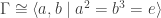
Using the fact that is a free product, we can think of the classifying space as the wedge sum of the classifying spaces and . These spaces are the homotopy quotients  of points (which we give two different names to make the diagrams we’re about to draw easier to parse) by the trivial actions of and . Intuitively, they can be thought of as “half a point” and “a third of a point,” respectively. We’re going to draw as their wedge sum using the following dessin (using QuickLaTeX, because WordPress doesn’t support xymatrix):

The reason we want to draw is that we’re going to think of finite index subgroups  as finite covers , and we’ll be drawing covers of this picture in a way closely analogous to how we can draw finite index subgroups of free groups by drawing covers of graphs.

What do covering spaces of this thing look like? The preimage of the edge will be a disjoint union of edges, so we expect to see something like a graph. The interesting question is what happens locally around the “orbifold points” . The covering space theory of these spaces is very simple: they both admit a single nontrivial connected cover, namely points (a double and a triple cover, respectively), and every covering space is a disjoint union of some copies of these nontrivial covers and the trivial cover. (This reflects the corresponding decomposition of -sets resp. -sets into transitive components.)

What’s more interesting is how the edge and the orbifold points interact. When gets covered by in some cover, the portion of the edge adjacent to it is doubled; similarly, when gets covered by in some cover, the portion of the edge adjacent to it is tripled and acquires a cyclic ordering (which describes how acts on the fiber over a basepoint in ).

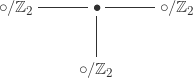
For example, here is the unique connected double cover of .

The orbifold point has “unfolded” itself into an ordinary point , in the process doubling the edge, but the orbifold point has no interesting double covers, so it can’t “unfold” yet.

We can extract a lot of information from this dessin. Recall that in order to get a subgroup of of a space from a cover of it, we need to pick both a basepoint and a lift of that basepoint to the cover. Here it’s easiest to pick a basepoint in the middle of the edge, where there’s no funny orbifold business going on, and so a lift of the basepoint corresponds to an edge in the cover. The conjugates of the subgroup we get come from picking different edges, and two edges give the same subgroup iff they are related by an automorphism of the cover. (Moreover, “automorphism of the cover” means more or less the obvious thing in terms of dessins; we’ll be more precise about this later.) In particular, we can see visually when a subgroup is normal: it’s iff the automorphism group of the corresponding dessin acts transitively on edges, which is the case here. More generally, the number of subgroups conjugate to a given subgroup is given by the number of orbits of the action of the automorphism group on the edges of its dessin.

After picking an edge, the corresponding subgroup of is given by the stabilizer of this edge with respect to the action of on edges given as follows: if we write as a free product

then sends an edge which is connected to an “unfolded” white point to the other edge connected to (and otherwise fixes the edge), and sends an edge which is connected to an “unfolded” black point to the next edge in the cyclic order (and otherwise fixes the edge). We can find a set of generators for the stabilizer by finding a spanning tree of the dessin (which is unnecessary here) and looking at the corresponding loops we get in the same way as in the case of graphs, while remembering that there are extra loops coming from and .

More topologically, this procedure computes the (“orbifold”) fundamental group of the dessin, regarded as a picture of a space (“1-dimensional orbifold”) obtained by gluing copies of and to some of the vertices of a graph, via iterated application of Seifert-van Kampen.

(This argument, cleaned up and made fully rigorous, shows that every subgroup of , not necessarily finite index, is a free product of copies of , and . For a generalization of this result to arbitrary free products, which you should be able to guess from here, see the Kurosh subgroup theorem.)

From this description we see that the unique subgroup of index in (which can be described as the kernel of the natural map killing the second factor) is the free product

.

Now let’s move on to index . Here there is an obvious triple cover, namely

given by “unfolding” but covering  trivially. (We need to pick a cyclic ordering of these three edges, but it doesn’t matter too much because the resulting dessins are isomorphic.) The corresponding subgroup is normal (as we can see because the automorphism group of this dessin acts transitively on edges); in fact it is the kernel of the natural map killing the first factor. This dessin shows that it is the free product

.

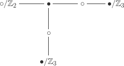
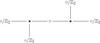
But we know that there are subgroups of index . The other are conjugate and come from the same dessin, namely

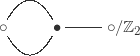
where has now also been “unfolded” once. The cyclic ordering on the edges around (which we haven’t drawn) matters now: without it this dessin would have a nontrivial automorphism exchanging the two edges around .

This is the first example we’ve looked at where the underlying graph is not a tree, and accordingly we get our first  factor in the free product decomposition: this subgroup (we’ll pick our basepoint to be the odd edge out) is the free product

.

We get the free generator from the loop in the dessin as follows: takes us from our basepoint to (depending on the cyclic ordering) one of the other two edges around . Going around the loop involves passing through , which corresponds to acting on one of the edges around using to get the other one. Finaly, going back to our basepoint involves passing through , which corresponds to using again.

As we’ll see later, this subgroup is in fact (conjugate to) the smallest congruence subgroup .

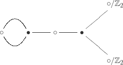
Let’s move faster now. The  subgroups of index form conjugacy classes of size coming from the following dessins, which have trivial automorphism group:

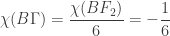
The dessins tell us that these subgroups are free products and respectively. The second one is (conjugate to) the second smallest congruence subgroup .

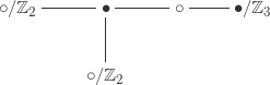
The subgroups of index form a single conjugacy class coming from the following dessin, which again has trivial automorphism group:

This dessin tells us that these subgroups are free products .

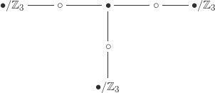
Index  is when things start getting exciting because we can now have two trivalent vertices : among other things, we see our first appearance of subgroups which are torsion-free (and hence free). The dessin

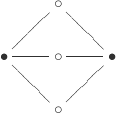
has both and fully “unfolded.” Abstractly the corresponding subgroups are free products (so free groups on two generators).

There are actually two dessins here depending on whether or not the cyclic orderings around the two copies of match, and they are not the same, although they both have transitive automorphism group and so correspond to normal subgroups. One of them corresponds to the kernel of the natural map

while the other corresponds to the kernel of the natural map

and hence to the congruence subgroup .

But there are also torsion-free subgroups of index that are not normal, coming from the dessin

which does not have transitive automorphism group. There are orbits of edges under the action of the automorphism group (which is , coming from the obvious reflection), so we get conjugate subgroups, one of which them is the congruence subgroup .

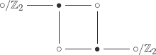
The congruence subgroup also has index , and its dessin is

so in particular it is not free: instead, it is the free product . This dessin has trivial automorphism group, so we get  conjugates.

There are  dessins left for index :

The first dessin here is actually dessins depending on whether the cyclic orderings match again. Altogether we find that there are conjugacy classes of subgroups of of index , with sizes (in order based on the order in which we drew the dessins)

in agreement with our previous count. This means that the sequence of conjugacy classes of subgroups of index in begins

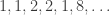
which we can look up on the OEIS, getting the sequence A121350.

Dessins as graphs

The graphs appearing here as dessins are bipartite graphs ( vertices can only be connected to vertices) where vertices have degree or and vertices have degree or . In addition, the vertices of degree are equipped with a cyclic ordering on their edges.

These dessins can be thought of as built up of copies of a single “puzzle piece,” namely an edge with “half a point” on one side and a “third of a point” on the other (perhaps a half and a third of a sphere, with appropriate connecting bits). The name of the game is that you take of these pieces and combine them by combining two half-points to make a whole point and three third-points to make a whole point . You can even encode the cyclic orders around the points by arranging the connecting bits so that three pieces can only connect in one cyclic order, and one of the connecting bits has an arrow pointing to the other. I wonder if someone would be interested in manufacturing these…

Euler characteristic

It’s not hard to see that torsion-free subgroups can only exist when the index is divisible by . This is because, thinking in terms of the corresponding transitive -sets , torsion-freeness is equivalent to both the generator of order and the generator of order acting with no fixed points. The first condition means is divisible by , while the second means is divisible by .

A more geometric way to see this is using the notion of virtual or orbifold Euler characteristic, which in some sense generalizes both the usual Euler characteristic and groupoid cardinality. We will only compute this number for (classifying spaces of) finitely generated groups which are virtually free, meaning that they contain a free subgroup of finite index (necessarily also finitely generated), which is the case for all finite index subgroups of . In this case the Euler characteristic is determined by the following two axioms:

•  , and
• If is a subgroup of of index , then .

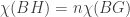Note that is the Euler characteristic in the usual sense of , which can be described as a wedge of circles. The second axiom is motivated by the fact that the map is an -fold cover.

Since has a free subgroup on two generators of index , its Euler characteristic is

.

But the Euler characteristic axioms also imply that if is a finite group, then (since is a subgroup of of index , and , being the free group on generators, has Euler characteristic ), and we can arrive at this formula in another way assuming that inclusion-exclusion holds in a suitable form for this notion of Euler characteristic: namely, is obtained by connecting  and by an edge, so if the usual inclusion-exclusion formula holds, then we should have

.

Assuming that Euler characteristic is well-defined, it now follows that a subgroup of of index has Euler characteristic , which is an integer iff is divisible by . Hence we learn not only that the free subgroups must have index but that they must be free on generators.

You can now go back through the examples above and verify that their Euler characteristics computed using either their index or inclusion-exclusion agree: for example, the unique subgroup of index has Euler characteristic

.

Drawing congruence subgroups

The dessins we’re drawing describe sets equipped with a transitive action of , namely the edges of the dessins, in the manner described above. For the congruence subgroups , the corresponding -set is given by the natural action of on itself, while for the congruence subgroups , the corresponding -set is given by the natural action of on the projective line .

may be a little unfamiliar if is not prime; for an arbitrary positive integer , it can be described as the quotient of the set of coprime pairs by the equivalence relation of multiplication by a unit in . Loosely speaking, these pairs can be thought of as fractions modulo , although if isn’t prime they have some funny and somewhat unexpected behavior. The size of , and hence the index of , is

and so we can compute that have indices respectively, and these are the only ones of index at most . The index of is the size of ; the only one of these groups of size at most is .

Here’s how to draw the dessin corresponding to . The generator of order can be taken to be the fractional linear transformation

acting on the elements of thought of as fractions as above, while the generator of order can be taken to be the fractional linear transformation

.

Since the action of is transitive, we can reach every element of by repeatedly applying each of these transformations to any particular point, say (by which we mean the ordered pair ). We can build up the dessin from here by repeatedly applying and and adding vertices and edges as appropriate.

For example, here is the dessin for drawn in this way, now with the edges labeled by elements of :

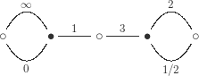
The implied cyclic order around the vertices, corresponding to the action of , is clockwise.

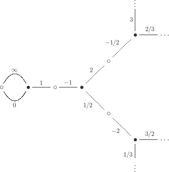
None of what we’ve said requires the subgroups to have finite index, so here is a small slice of the dessin for the subgroup generated by translation , which corresponds to the action of on the projective line (since translation generates the subgroup fixing ). The dessins are all quotients of this one.

Higher-dimensional pictures

Dessins give a “1-dimensional” picture of the finite index subgroups of the modular group in terms of certain 1-dimensional orbifolds modeling the classifying spaces . It is also possible to give 2-dimensional, 3-dimensional, and 4-dimensional pictures.

• In 2 dimensions, we can look at the quotient . These quotients are generalizations of modular curves, and their points describe elliptic curves equipped with various extra data. Geometrically they are 2-dimensional orbifolds which become ordinary surfaces if is torsion-free. Remarkably, Belyi’s theorem implies that in this case, the corresponding Riemann surfaces arise from algebraic curves defined over , and that all algebraic curves over arise in this way.
• In 3 dimensions, we can look at the quotient . These quotients are the unit tangent bundles of the modular quotients above, and are always ordinary 3-manifolds with PSL geometry. itself is the complement of the trefoil knot in , so the quotients  are finite covers of this complement. See this blog post by Bruce Bartlett for more on this.
• In 4 dimensions, we can look at the quotient 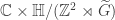, where denotes the preimage of in . (I won’t write out this action because I have very little to say about this construction.) These quotients are elliptic surfaces with base and fiber over a point the elliptic curve corresponding to that point. Elliptic surfaces arising in this way are called elliptic modular surfaces.

We can recover dessins as drawn above from the modular curves as follows (although these are not quite the dessins described in the Wikipedia article, which I believe come from finite index subgroups of rather than ). These curves come with a natural map , where is the usual modular curve parameterizing elliptic curves with no extra structure. There is a map

sending an elliptic curve 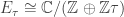(where ) to its j-invariant which is almost an isomorphism. However, the action of on is not free, so we shouldn’t just take the ordinary quotient: the moduli space of elliptic curves is really a stack, and we can think about this stacky structure in terms of two special “orbifold points” in the quotient .

One of these special points corresponds to the elliptic curve given by quotienting by the square lattice, which has an extra automorphism of order given by multiplication by , while the other corresponds to the elliptic curve ( a primitive sixth root of unity) given by quotienting by the hexagonal lattice, which has an extra automorphism of order given by multiplication by . These extra automorphisms are reflected in the fact that these points have nontrivial stabilizers under the action of . Namely, the generator of order stabilizes , and the generator of order stabilizes .

So we can draw the dessin for itself as a path in (say a geodesic with respect to the hyperbolic metric) connecting the two special orbifold points. The preimage of this path in for a subgroup (not necessarily finite index) of is then the dessin associated to . When the corresponding dessin is a tree sitting inside (I think it is half of the 1-skeleton of the usual tesselation of the hyperbolic plane on which acts by symmetries), and this tree can in fact be used to prove that .

It follows that if is torsion-free, then the dessin of can be drawn on a surface whose genus it is possible to calculate. In the simplest case this surface has genus zero and is a punctured sphere; the corresponding dessins are then planar. This is the case, for example, for the modular groups 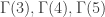, where the corresponding dessins encode Cayley graphs for the groups

.

These dessins turn out to be essentially 1-skeleta of the tetrahedron, cube, and dodecahedron respectively. More precisely, the dessins can be obtained by coloring the vertices of the 1-skeleta , then adding a to the middle of each edge (and then cyclically ordering appropriately).